Explicit Context Mapping for Stereo Matching

Abstract

Deep stereo matching methods usually conduct the matching process in the low-resolution space to reduce the computational burden. However, mapping the disparity map from the low-resolution (LR) space to the high-resolution (HR)space causes loss of details. Many efforts have been paid to develop additional refinements to recover details. This paper proposes an explicit context mapping method that directly preserves details during the mapping process. We formulate the mapping as Bayesian inference, where we deem the disparity map in the LR space as the prior and that in the HR space as the posterior. We present the explicit context, which is defined as the similarity between their and LR disparity maps to realize the inference. Specifically, we build an explicit context mapping module that seamlessly integrates with stereo matching networks without modifying original network architectures. Experiments on the Scene Flow and KITTI 2012 datasets show that our method outperforms the state-of-the-art methods.

Problem

The current top-down, bottom-up network structure is generally realized by the auto-encoder structure. The sub-sampling operation provides the regional feature with a large receptive field, but it also brings the loss of details like silhouettes. Using skip-connection to bring back the high-resolution feature map can maintain the details. However, it is hard to interpret how the low-level matching result is refined by the high-level features.

Solution

We propose to explicitly model the mapping relation by the similarity between high-resolution (HR) and low-resolution (LR) feature maps. The mapping relation is represented by a weight matrix where each element is the similarity between corresponding HR and LR feature vectors. To map the LR matching result back to HR space, we use this matrix rather than use the normal up-sampling layers like bilinear interpolation or deconvolution.

Figure 1. The below figure shows the explicit context mapping for the disparity map.

For the one connected mapping, each low-resolution value only influences high-resolution values in the mapped region (red), where the same color indicates correspondences. For the four connected mappings, each low-resolution value would influence not only the mapped region (red) but also the four connected regions (blue)

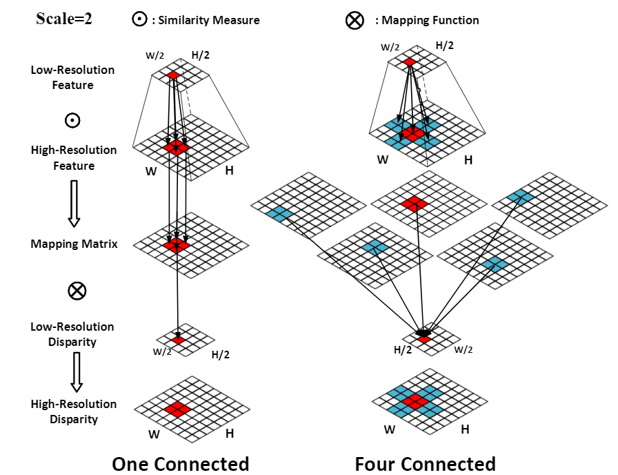
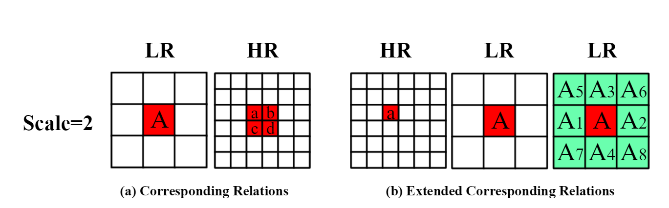
Figure 2. The below figure illustrates the correspondence between LR and HR space when the scale is 2.

(a) The LR disparity value at position 'A' corresponds to four HR disparity values at positions 'a', 'b', 'c', and' (red color). (b) We take the disparity at position 'a' as an example. The HR disparity value at position 'a' corresponds to the LR value at position 'A' (red color). Its eight-connected values are at 'A1',....'A8' (green color). High-resolution disparity at positions 'b', 'c', 'd' have the same corresponding relations as 'a'.

Result

Table 1. The result on the SceneFLow dataset.

Table 1 shows our method gets the lowest end-point-error. Compared to the baseline PSMNet, we get a promotion of 0.22 by mapping the disparity map. And the promotion is more significant by mapping the cost volume that reaches the 0.59 EPE and more than 0.4 lower than the baseline.

Table 2. The ablation result on the SceneFLow dataset.

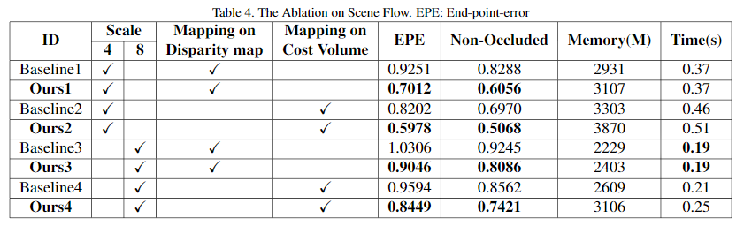
From Table 2, we can see our method can effectively improve the accuracy while barely add the computational cost. Comparing the EPE on the whole image and the non-occluded areas shows that our method performs better on the non-occluded areas. This result indicates that our method is a kind of refinement of the right matching result from the low-resolution space, but it cannot rectify the wrong matching results. Therefore, we get a higher error on the occluded areas where the right matching results do not exist. By comparing the results with different scales, we can see our method gets better results on a smaller scale, where one LR feature corresponds to fewer HR features. However, even for the large scale, the promotion is still obvious close to 0.1 EPE. We also validate our method separately on the disparity map and cost volume; mapping the cost volume takes more memory and time and provides a lower error close to 0.1 for both scale.

Figure 3. The visualization of the explicit context mapping result.

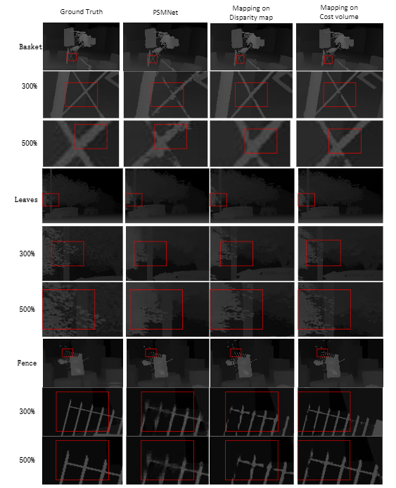
We illustrate the SceneFlow benchmark result by three classes of rich details, i.e., basket, leaves, and fences. In the 500% scale result, we can see the details are maintained with the context mapping. Our method bridges the gap in the PSMNet result and gives a clear shape to model the contours. In fragile areas or small objects, it can give a much better result. Although these objects only take lower than 1% of the whole image, these results are important references for the 3D scene reconstruction. Besides, we also compare the mapping performance on the disparity and cost volume. As the disparity map has lost the information to rectify the result, mapping the cost volume gives a much better visual result for the thin structure objects.

Table 3. The result on KITTI12 dataset.

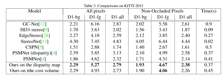
Table 4. The result on the KITTI15 dataset.

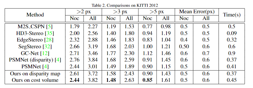
It is a little pity that we re-train the PSMNet on the KITTI but cannot get reported results, this might come from the augment method during training. We use the re-trained model as the baseline, which is the PSMNet(disparity) in the table. The promotion is not as obvious as in the SceneFlow, which is only about 0.3 EPE on the KITTI2015. The main reason for the limited promotion is that KITTI's supervision is a sparse disparity map, which makes the gradient back to the mapping matrix during the backward training is unconstrainted. Therefore, the mapping matrix lacks information to learn the correct correspondence. Besides, with limited supervision, the network is easier to find the shortcut and thus get a limited generalization performance. This conclusion is supported that we observe that after 50 epochs, our method gets a lower loss than the baseline PSMNet, but the testing result is higher.