Interpretable stereo matching with region support

Abstract

The application of CNN achieves great success on the stereo matching. But most methods implicitly use neural networks for stereo matching, which is difficult to solve a particular challenge such as occlusion or textureless areas. In this paper, we propose the region support to handle these challenges in stereo matching explicitly. The region support is an extension of the traditional variable support, enhanced by a novel learning scheme. The learning-based region support is obtained by a novel coarse-depth inference network i.e., the region support network, which infers the depth from a single image. Besides, we propose improved cost computation, cost aggregation, and refinement methods, which are reformulated by region support. The final reformulated stereo matching pipeline reaches remarkable performance both on speed and accuracy. The experiments on SceneFlow and KITTI demonstrate the effectiveness of the region support.

Problem

Current deep stereo matching methods are mostly built in a black box and lack of interpretability. To build a reliable stereo matching pipeline, we argue that it is essential to design the network in an explainable manner. Therefore, we propose to use the regional guidance, i.e., region support, to regularize the intermediate network output and help us interpret the stereo matching process.

Solution

We propose the region support knowledge as guidance to regularize the deep stereo matching. The region support knowledge,$P$, consists of four kinds of prior knowledge, where $P_{1}$ is the discriminative region supports, $P_{2}$ is the representative pixel sets, $P_{3}$ is the object-level segmentation, and $P_{4}$ is the plane-level segmentation. To tackle the tradeoff of smoothness and details, the $P_{1}$ knowledge is endued with the ability to distinguish the pixels' discriminability, so the representation of pixels can have relevant context information corresponding to their discriminability. The $P_{2}$ knowledge that evaluates the representativeness of the pixels reduces the redundant cost computation by only matching the representative pixels and leaving the others to the aggregation. The $P_{3}$ knowledge is the object-level segmentation, which can constrain the matching points' searching space by the object-level disparity from the pre-matching between objects in the stereo pair image. Last, but certainly not least, the plane-level segmentation of the $P_{4}$ knowledge reveals whether the pixels are at the same depth. This knowledge directly offers guidance from depth information for the aggregation. Accordingly, complex aggregation can work fast and reliably.

Figure 1. The pyramid cascade network is presented to extract our region support knowledge

The network can be split as four stages, each of which determines a kind of region support knowledge. A shallow network is first used to generate the full-resolution feature map (Conv-feature) to determine the $P_{1}$, and then we use a pyramid pooling unit to get the multi-scale feature (pyramid-feature). Both the two kinds of features are shared for the other three stages. But each stage has its unique fused feature by combining the result of the former stage with the shared feature. The clustering operation is employed on these fused features to determine the $P_{3}$ and $P_{4}$. Both the $P_{3}$ and $P_{4}$ are used as masks to constraints the later stage working among certain regions. The final stage determines the $P_{2}$ from the $P_{4}$ by finding out the representative pixels among each plane. The loss functions for $P_{1,2}$ are the two class cross-entropy, and the loss functions of $P_{3,4}$ is the discriminative loss for clustering. These four-loss functions are fused with different weights to form the final joint training loss.

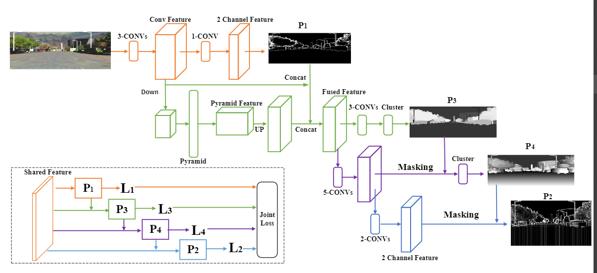
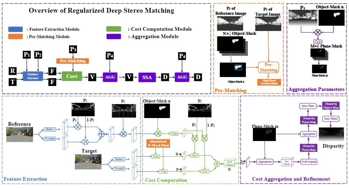
Figure 2. The regularized deep stereo matching.

In the overview frame, we can see the region support knowledge offers regularizations for each step of the stereo matching. The $R$ and $T$ corresponds to the reference image and target image. The $F$ is the extracted feature. The detailed operation is shown in the feature extraction module with blue color, where we employ two feature extractor to obtain the feature for each pixel and use the $P_{1}$ to fuse the feature. The $P_{2}$ gives a sparse shape of the feature map where we only hold the representative pixels. Then the $P_{3}$ guides the pre-matching module, which is shown in orange color. The obtained pre-matching result constraints the searching space of the cost computation, which is shown in green color. The cost computation step is finally accomplished by employing the correlation similarity measure separately on the two kinds of the feature. After that, we get the cost volume $V$ and use the $P_{4}$ to determine the aggregation parameters. The aggregation module is shown in purple color, which is both used for cost aggregation and refinement. A sparse soft-argmin (SSA) is presented to compute the disparity map from the cost volume. Since the cost computation and aggregation carry out independently on each object and each plane, we adopt two sum modules to obtain the unabridged disparity map.

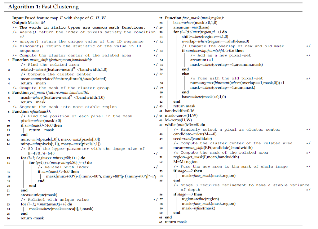
Algorithm 1. The fast clustering algorithm to compute the region support knowledge

Rather than using the proposal based method to carry out the segmentation task, we design a cluster layer to determine the region support division. The reason is that the number of object instances varies a lot in different scenes, and the supervision for these semantic or instance labels always lacks in the stereo dataset. Furthermore, the proposal based methods can not handle the segmentation with the labels by depth for each region because they are infinite and not constant in different scenes. Therefore, we propose a fast clustering algorithm as an additional layer for stages 2 and 3 to determine the division of region supports for the next stage. The fast clustering algorithm is shown in Algorithm 2. The algorithm is designed based on the mean-shift cluster, which consists of two steps: clustering and mask generation. Instead of iteratively use the mean shift until it coverages, we only compute the cluster center twice, and in the second time, we use the shifted cluster center to generate the initial mask. Then the initial mask fuses with the previously obtained mask after each iteration. An additional refining operation is also used to determine $P_{4}$ before the mask fusion, where we constrain each related areas by a maximum size of $80\times80$. The proposed clustering algorithm is fully differentiable, but we freeze them during backpropagation because the gradient during clustering operation will confuse the joint training and bring a great computational burden. The clustering only offers the generated masks for the later stage's masking operation, as for the training, we adopt a discriminative loss.

Experiment Result

Data Preparation

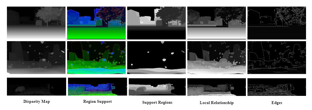
This Figure shows the obtained region support. The region support has three channels, which are support regions, local relationships, and edges. The stereo matching methods require three instructive guidance. Since the region support is learning-based, we extract the region support from the disparity map for the training purpose. During training, the obtained region support from disparity is used as the ground-truth of the RSN and the initial region support for the stereo matching network. After training the region support network, we replace the region support for stereo matching with the learned region support from the RSN. To obtain the ground-truth, we extract the region support The first channel is the support regions, each of which is consisted of pixels in similar disparity. We apply the Felzenszwalb’s efficient graph-based segmentation to the disparity map to obtain the initial support regions. After that, we apply an aggregation operation between the regions according to the disparity continuity. Then we divide the aggregation results into 32 sets according to the average disparity, which is the final support regions. The second channel is the local relationship. It is the combination of the results of original Felzenszwalb’s segmentation and Sobel edges detection. The third channel is the edges in disparity space, which is obtained by the canny edge detection and Sobel detection.

Benchmark Performance

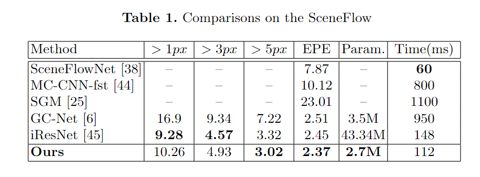
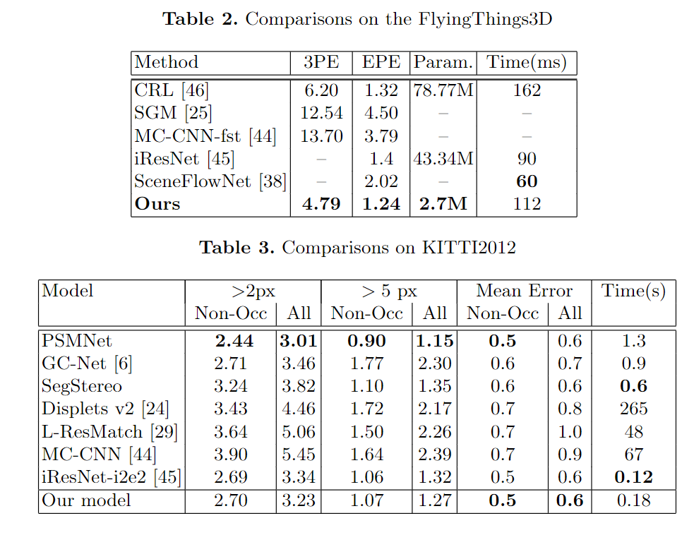
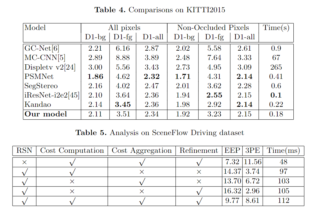
We test our stereo matching method on two datasets: SceneFLow and KITTI. The SceneFlow is a synthetic dataset that consists of three datasets Driving, FlyingThings3D, and Monkaa. These three datasets are constructed in different scenes. The Driving dataset is a mostly naturalistic street scene from a driving car's viewpoint, made to resemble the KITTI datasets. It has 8830 training images that we use to analyze region support's effectiveness, and the results are shown in Table.1. The average evaluation of SceneFlow is shown in Table.1. We compare with SceneFlowNet, GC-Net, iResNet, and MC-CNN, where we reach the best performance on $5px$ error rate and endpoint error(EPE) with the smallest model parameter. The evaluation of FlyingThings3D is shown in Table.2. Compared to CRL, iResNet, and SceneFlowNet, we reach the best performance on EPE and 3PE. The endpoint-error(EPE) is the average Euclidean distance between the prediction and ground-truth, and the three-pixel-error(3PE) is the percentage of EPE value more than 3. The KITTI dataset is the real scene dataset on a driving car. The KITTI dataset contains 194 training and 195 test image pair consisting of images of challenging and varied road scenes obtained from LIDAR data. We use the pre-trained model on the Driving dataset and fine-tune on KITTI to obtain the final model. The comparison with GC-Net, PSMNet, SegStereo, iResNet-i2e2, MC-CNN, Displetv v2, and Kandao are shown in Table.3 and Table.4. From the evaluation, we can see that the proposed method reaches the state-of-art performance both on KITTI2012 and KITTI2015.